Assignment
Given the interdisciplinary and strongly practical nature of Multimedia Retrieval (MR), the course is assessed by means of a practical assignment rather than a classical written exam. This allows students to
- build up practical skills in choosing, customizing, and applying specific techniques and algorithms to construct a realistic end-to-end MR system;
- learn the pro's and con's of different techniques, and also subtle practical constraints these have, such as robustness, ease of use, and computational scalability;
- make concrete design and implementation choices based on real-world output created by their system;
- get exposed to all steps of the MR pipeline (data representation, cleaning, feature extraction, matching, evaluation, and presentation);
- learn how to present their results at academic level in a technical report.
Important: Before you start working, read this entire page, as well as the pointers given in the Additional material.
Structure
The assignment reads very easily:
Build a content-based 3D shape retrieval system that, given a 3D shape, finds the most similar shapes in a given 3D shape database
The assignment execution is organized as a sequence of steps, in line with typical software engineering design-and-implementation principles. Early steps are quite easy. Subsequent steps are more complicated and build atop the earlier ones. These are as follows:
Step 1: Read and view the data (1 point)
Outcome
Build a minimal application able to read and visualize 3D mesh files
Aims
Familiarize yourself with the 3D shape database(s) at hand, the types of shapes they contain; choose your source-code development tools; use these to build the skeleton of a minimal 3D shape processing application, which you will extend in the following steps.
Description
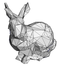
Start having a look at the two shape databases provided as example, the Princeton Shape Benchmark and the Labeled PSB Dataset (both described here). Download a few shapes from the chosen database, making sure you have at least one in the PLY format and one in the OFF format. Next, implement a minimal program that allows you to read the shape and display it as a shaded model, with or without cell edges drawn. The program should also allow you to visually inspect the shape, i.e., rotate the viewpoint around it, zoom in/out, and pan (translate).
Check that your program works OK with both PLY and OFF shapes. You have two options here:
- either implement readers for both the PLY and OFF file formats
- use a converter from one format to the other, which you first run before reading the shapes (preferred)
Pointers
- Module 3: Data representation
- GeomView tool, allows you to check/view your 3D shapes before doing anything with them
- MeshLab tool, implements similar functionality to GeomView, but also mesh refinement and simplification
- OpenGL crash course, including how to build a simple PLY viewer
- OFF mesh tools
- Triangle mesh tools
- Description of the Princeton and Labeled PSB Databases
Step 2: Preprocessing and cleaning (1 point)
Outcome
Prepare your shape database so it's ready to be used for the next step, feature extraction. This means carefully checking that all contained shapes obey certain quality requirements and, if not, preprocessing these shapes to make them quality-compliant.
Aims
Familiarize yourself with the various problems that 3D meshes may have (in the context of MR); how to detect these problems; and how to fix these problems. Familiarize yourself with building and/or using simple tools to process 3D meshes. Familiarize yourself with the formats in which the Princeton Shape Benchmark or the Labeled PSB Dataset are stored.
Description
Start building a simple filter that checks all shapes in the database. The filter should output, for each shape
- the class of the shape
- the number of faces and vertices of the shape
- the type of faces (e.g. only triangles, only quads, mixes of triangles and quads)
- the axis-aligned 3D bounding box of the shapes
Shape class: All shapes in the Princeton and Labeled PSB Datasets come with a class label. There are several classifications provided there. For the Labeled PSB database, use the classification which divides shapes into 19 classes (aircraft, animal, etc). For the Princeton database, you have multiple levels of detail (granularities) of classification. Use the middle one which divides shapes into (roughly) 45 classes. For each shape, read and store the class ID in your shape database. We will use the class labels later on in Steps 5 and 6.
Use the output of the filter, e.g. saved in an Excel sheet or similar, to find out (a) what is the average shape in the database (in terms of size and cell types); and (b) if there are significant outliers from these average (e.g. very large or very small sizes in terms of number of cells/vertices). Use the viewer constructed in step 1 to visualize an average shape and these outliers (if any).
Next, if outliers contain poorly-sampled shapes (having under 100 vertices and/or faces), you need to refine these, so that feature extraction (next step) will work well. Refinement means splitting large faces into smaller ones. There are several ways to refine a mesh:
- use the MeshLab tool; it contains many ready-to-use refinement methods! However, this may be a bit tedious, since you have to invoke refinement manually;
- use the OFF mesh tools package. This allows refining many meshes easily in a batch process. However, carefully experiment with refinement options so that you obtain meshes which are (a) correct and looking close to the original ones and (b) not too large (over 50K vertices/faces is considered too large).
Check the refinement results by using your 3D viewer and statistics tools developed so far in the assignment. After refinement is done, save a print-out of the refined-database statistics, showing the new values for the refined meshes.
Finally, design a simple normalization tool. The tool should read each shape, translate it so that its barycenter coincides with the coordinate-frame origin, and scale it uniformly so that it tightly fits in a unit-sized cube. Run your statistics computation (see above) to show that the normalization worked OK for all shapes.
Important note
Processing the entire Princeton or PSB databases can be very challenging! These contain hundreds of shapes in multiple classes. A good way to proceed with the assignment is to first consider a reduced database. The key constraints here are that (a) the reduced database should contain at least 200 shapes; (b) you should have shapes of most (ideally all) of the existing class types in the database; (c) try to balance the classes, i.e., do not use tens of models of one class and only a handful of models of another class.
Pointers
- as for Step 1
Step 3: Feature extraction (2 points)
This is likely the most challenging assignment step! Make sure you allocate it enough time
Outcome
Extract several features from each shape in your preprocessed 3D shape database. Save these features in a tabular form (e.g. in a table where each shape is a row and each feature is a column). Add the functionality to your program to load a given shape and extract and print its feature values (or, if feature values have already been computed for this shape, retrieve and print these).
Aims
Familiarize yourself with several types of features and methods to compute (extract) these from 3D shapes; learn how to robustly use these methods in terms of preparing shapes for extraction and normalizing the extracted features for further inspection; understand how discriminant features are for different types of shapes.
Description
This step consists of two sub-steps, the second of which allows for two options:
Step 3.1: Full normalization
Implement the four-step normalization pipeline described in Module 4: Feature extraction. You have already implemented centering and scaling in Step 2. Now you need to add:
- alignment: Compute the eigenvectors of the shape's covariance matrix using PCA and align it so that the two largest eigenvectors match the x, respectively y, axes of the coordinate frame;
- flipping: Use the moment test to flip the shape along the 3 axes (after alignment).
Use your viewer to check that the entire 4-step normalization works OK.
Step 3.2 (variant A): 3D shape descriptors
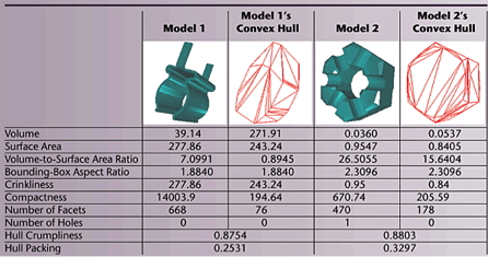
Compute the following 3D elementary descriptors presented in Module 4: Feature extraction:
- surface area
- compactness (with respect to a sphere)
- axis-aligned bounding-box volume
- diameter
- eccentricity (ratio of largest to smallest eigenvalues of covariance matrix)
Note that the definitions given in Module 4 are for 2D shapes. You need to adapt them to 3D shapes (easy).
All above are simple global descriptors, that is, they yield a single real value. Besides this, compute also the following shape property descriptors:
- A3: angle between 3 random vertices
- D1: distance between barycenter and random vertex
- D2: distance between 2 random vertices
- D3: square root of area of triangle given by 3 random vertices
- D4: cube root of volume of tetrahedron formed by 4 random vertices
These last five descriptors are distributions, not single values. Reduce them to a fixed-length descriptor using histograms. For this, compute these descriptors for a given (large) number of random points on a given shape (you see now why you need to have finely-meshed shapes?). Next, bin the ranges of these descriptors on a fixed number of bins B, e.g., 8..10, and compute how many values fall within each bin. This gives you a B-dimensional descriptor.
Step 3.2 (variant B): 2D appearance-based elementary descriptors
Warning: This step requires a good mastery of OpenGL
Instead of using 3D descriptors, you will now use 2D descriptors. For this, you need to first extract a silhouette image of the 3D shape. For this, render the shape aligned along its major and medium eigenvectors (as done by the 4-step normalization). While rendering, use a white background and switch off all lighting, so your shape is rendered black. Next, grab the frame buffer image and save it as a black-and-white image file. Next, use this image to compute the following 2D shape descriptors:
- area (number of foreground pixels)
- perimeter (number of foreground pixels neighbor with at least 1 background pixel)
- compactness
- axis-aligned bounding box
- rectangularity
- diameter
- eccentricity
- length of 2D shape skeleton / length of 2D shape perimeter
For this, you can use directly the definitions given in Module 4: Feature extraction
Important notes for step 3
- start experimenting with just a few shapes, e.g., some of the simpler ones in your database. Check that you can compute the simplest descriptors on them: Since these descriptors are pretty intuitive, you can directly check if your code outputs correct values (think e.g. of rectangularity or eccentricity, easy to check on simple shapes like a cube or a sphere for which you know the ground-truth). Only when this works do consider the more complex shapes.
- if your code cannot handle certain shapes in the database, mark them as such, mention this in your report, and just skip them from the computations. Don't get blocked trying to fix computing some descriptor that won't work on just a few shapes!
Pointers
Step 4: Querying (2 points)
Outcome
In this step, you implement the first end-to-end querying system: Given a test shape, you extract its features (following the steps described in Step 3). Then, you compute the distances between these features and those extracted from all the shapes in the database (see again Step 3). You finally show to the user which are the best-matching shape(s). All in all, a simple implementation of a Content-Based Shape Retrieval (CBSR) system.
Aims
Familiarize yourself with matching: selecting a distance metric; computing distances between feature vectors; interpreting these distances to select next a good subset of matching shapes; and presenting these to the end user in an intuitive way.
Description
First, you need to normalize the extracted features from both your query shape and the shape database. Since different features may have different ranges (min..max values), you need to first bring these ranges to a common denominator. This way, features can be next safely used as components of a distance metric. For normalization, consider both min..max normalization and standardization (per feature: subtract average of values, for that feature, computed over the entire database, and divide result by standard deviation of that feature). Adapt your code so that it stores and displays the database of normalized features, so they can be easily inspected.
Next, consider which distance function you want to use. Several options are possible
- Euclidean distance
- cosine distance
- Earth mover's distance
Start with the Euclidean distance, which is easiest to implement and test, and fastest to compute. If this yields poor results, consider using other distance metrics, e.g., Earth mover's distance for comparing histogram features.
Implement a simple interface for querying:
- user picks a shape in the database (or alternatively can load a 3D mesh file containing a shape which is not part of the database; note that you can do this easily by simply selecting several shapes, from the benchmarks mentioned in Step 2, and not including them in the database)
- extract features of the query shape (if not from the database)
- compute distance of query shape to all database shapes
- sort distances from low to high
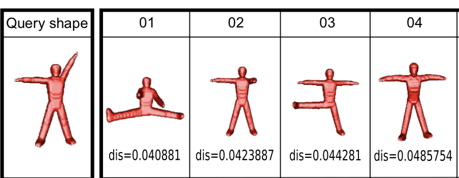
- present the K best-matching shapes, plus their distances to the query, in some visual way so the user can inspect them. Alternative: set a distance threshold t and present all shapes in the database having a distance to the query lower than t.
Notes
- keep it simple: Do not develop a too complex GUI or similar for querying and result presentation. Just stick with the minimal implementation allowing to specify a query shape and inspect the query results.
- keep it fast: If distance computations become slow, consider using a smaller database (eliminate some shapes from the database).
Pointers
Step 5: Scalability (2 points)
Outcome
In this step, you refine the design of your CBSR system to work faster with large shape databases. You use two mechanisms for this:
- a K-nearest neighbors (KNN) engine to efficiently find the K most similar shapes to a given shape
- a dimensionality reduction (DR) engine to reduce dimensionality of the feature vectors
Aims
Familiarize yourself with using KNN data structures to efficiently query large feature spaces; understanding the difference between using K-nearest neighbor search and R-nearest neighbor (range) search; understanding how to perform dimensionality reduction and how to use the resulting scatterplots.
Description
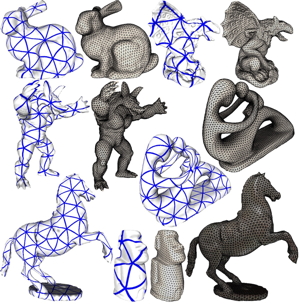
Take the feature database (all feature vectors computed for all shapes in the database, already constructed in Step 3) and construct a spatial search structure for it. For this, use the Approximate Nearest Neighbor (ANN) library (see Pointers below). Next, given a query shape, modify the simple query mechanism built in Step 4 to return the K-nearest neighbors or the R-nearest neighbors (where K and R are user-supplied parameters), using ANN. Display the query results using the same mechanism as built for Step 4.
Bonus point
This step is not mandatory. However, if you execute it (correctly), you gain an extra point. This is useful e.g. to obtain a higher grade, assuming that you would not get the entire points for some of the other steps.
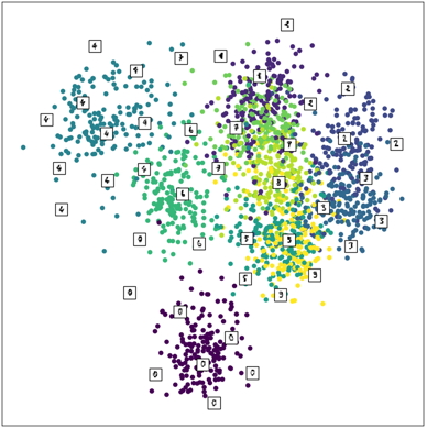
Take the feature database and perform dimensionality reduction (DR) on it, with 2 as target (embedding) dimension. That is, reduce your feature space to a 2D space. For this, the best option is to use the t-SNE DR engine (see Pointers below). The output will be a 2D scatterplot where every point is a feature vector and, implicitly, a 3D shape. Display the scatterplot and implement some minimal interaction mechanism to allow brushing a point - that is, indicating it by the mouse and displaying details about the underlying shape like the shape name and class. Also color the points by their class value. You read this value in your shape database in Step 2.
Notes
As for Step 4, keep the implementation of this step minimal so that it achieves its intended functionality. Do not implement complex GUI features for displaying the search results or the dimensionality reduction.
Pointers
- Description of the Princeton and Labeled PSB Databases
- t-SNE implementation
- Approximate Nearest Neighbors (ANN) implementation
- Module 8: Scalability
Step 6: Evaluation (2 points)
Outcome
In this step, you evaluate the performance of your CBSR system. Given each shape in the database, you query for similar shapes (e.g. using the K-nearest neighbors option implemented in Step 5). Next you check how the class IDs of the K items returned by the query match the class ID of the query shape itself. From this information you infer quality metrics for your CBSR engine.
Aims
Familiarize yourself with computing quality metrics for CBSR; choose a suitable metric to evaluate; evaluate the metric and display and discuss its results.
Description
Class IDs of the shapes in the database are key to understanding how to evaluate your CBSR system. Simply put: When querying with each shape in the database, the ideal response should list only shapes of the same class. When enough items are allowed in the query result, all shapes of the same class should be returned as first elements of the query.
To implement this step, choose an appropriate quality metric to implement. Options include
- accuracy
- precision, recall
- specificity, sensitivity
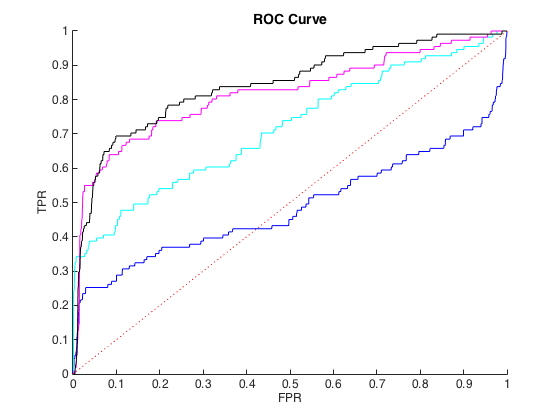
You only need to implement a single quality metric. Motivate your choice and describe how you implement the respective metric based on how the query system works (you provide a query shape and number K, you get K shapes in return). Compute next the metric for all shapes in the database. Present the metric results by aggregating it for each class individually and also by computing a grand aggregate (over all classes). Discuss which are the types of shapes where your system performs best and, respectively, worst.
Pointers
- Module 7: Evaluation
- Description of the Princeton and Labeled PSB Databases On this webpage, code is provided for computing and plotting various quality metrics. Study the code to see which parts thereof you can reuse, and how.
Deliverables
To complete the assignment, you have to
- deliver a written report describing the design and modeling choices made, and showing representative results of each step of your application (tables, snapshots, graphs);
- deliver the source code of the implementation of your assignment;
- hold an oral presentation demonstrating how your system works.
These deliverables are discussed below:
Report
The report should follow the typical organization of a scientific report:
- introduction, presenting the problem at hand; the constraints under which you work; and how the remainder of the report is structured;
- per assignment step, one section clearly describing what are the aims of the respective step; which design and modeling decisions you took to realize the step; and evidence demonstrating the results obtained in the respective step (e.g., in the form of tables, graphs/charts, or actual snapshots taken from the system)
- a discussion giving an overall assessment of the entire system, highlighting its strong points, and possible limitations (including their causes and potential solutions, even if these have not been implemented)
- a list of references containing pointers to all algorithms, papers, and tools used in the system's design and implementation
General writing guidelines:
- be precise: Wherever possible, use mathematical notations and equations to describe how your system operates instead of possibly vague plain text;
- be complete: cover all important decisions, including, for example, parameter settings;
- be honest: when certain functions do not work as desired, or certain datasets do not get processed, just report this. You will not lose points if you explain when and why this happens and the problem is not ascribed to a mistake in your implementation.
- make it replicable: indicate as many details as needed to make your work understandable. A good rule of thumb: Imagine you read the report (written by someone else). How much info do you need to understand and replicate what was done?
- be visually rich: CBSR is all about multimedia data! Hence, illustrate your work with graphs, snapshots, charts, to make it easy to follow and information-rich.
- be concise: You do not need to discuss coding details in the report. The source code (see below) does provide this information.
- report length: It is hard to give an optimal size for the report, given that different people write differently, use different document templates, and image sizes and pagination can make huge differences. However, in general, a good report for this course should contain not less than 25 pages.
Source code
The source code you deliver should allow one to easily replicate your work and findings.
For this, you need to provide minimally an archive (ZIP file) containing
- the full source code of your project, including 3rd party libraries. You can code in any mainstream programming language (e.g. C/C++, Java, Python, or a mix of those).
- a very short README file explaining how to build your code and how to run it.
- your shape database and extracted feature database (in any format you like, provided that your CBSR tool is able, of course, to read/write this format).
Presentation
The course ends with a mini-symposium during which all students get a slot to present their work. Ideally, your presentation should contain a live demo of your CBSR system showing how you accomplished all steps of the assignment. If desired, you can also have accompanying slides (this is a good idea in case your live demo does not work for whichever reasons). Questions are allowed from both the lecturer (obviously) but also other students participating to the symposium!